What & why Pandas?

Pandas is an open-source Python library that helps people work with and analyze data easily. It provides tools and functions to organize, clean, and manipulate data more conveniently and efficiently. Pandas make it simpler to work with data, even if you're not a coding expert.

Pandas primarily revolve around two core data structures: Series and DataFrame

What is Series?

A Series is a one-dimensional labeled array that can hold data of any type (integer, string, float, etc.). It is similar to a column in a spreadsheet or a single column in a table. The Series object consists of two main components: the data and the index.

The data component of a Series holds the actual values (data), which can be accessed using numerical indices or labels.The index component labels each data point, providing a unique identifier for each entry in the Series.

How to create a series:

import pandas library

import pandas as pd

To create a Series in pandas, use the pd.Series() function.

# Create a Series from a list
data = [10, 20, 30, 40, 50]
series = pd.Series(data)
print(series)

output:

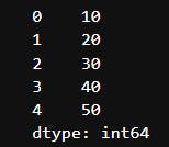
In the above example, we created a series from a list of integers. The resulting Series contains the values from the list, and each value is assigned an index (by default, a numeric index starting from 0).

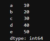
You can also specify custom index labels, by passing a list of labels as the index parameter:

# Create a Series with custom index labels
data = [10, 20, 30, 40, 50]
cust_index = ['a', 'b', 'c', 'd', 'e']
series = pd.Series(data, index=index)
print(series)

output: Series with custom indexes

What is DataFrame?

In pandas, a DataFrame is a two-dimensional labeled data structure that resembles a table or a spreadsheet. It consists of rows and columns, where each column can hold data of different types (e.g., numeric, string, boolean, etc.).

A DataFrame can be thought of as a collection of Series objects, where each column is a Series.

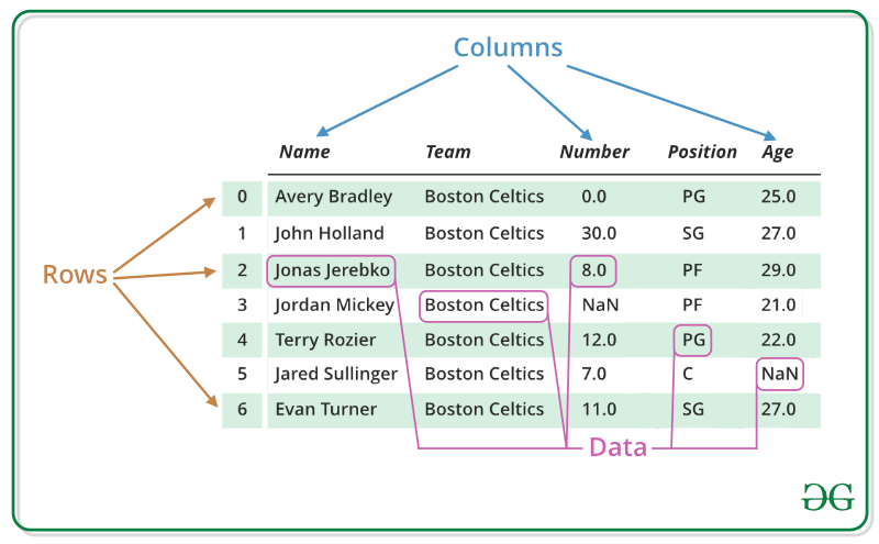
Image source: GeeksforGeeks

Creating a DataFrame:

# Create a DataFrame from a dictionary
data = {'Name': ['John', 'Alice', 'Bob'],
        'Age': [25, 30, 35],
        'City': ['New York', 'Paris', 'London']}

df = pd.DataFrame(data)
print(df)

Output:

In the above example, we created a DataFrame from a dictionary where the keys represent column names ('Name', 'Age', 'City') and the values represent the corresponding data. Each key-value pair in the dictionary becomes a column in the DataFrame, and the values are aligned based on their positions.

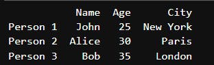
You can also specify custom index labels for the rows using the index parameter:

# Create a DataFrame with custom index labels
data = {'Name': ['John', 'Alice', 'Bob'],
        'Age': [25, 30, 35],
        'City': ['New York', 'Paris', 'London']}

index = ['Person 1', 'Person 2', 'Person 3']

df = pd.DataFrame(data, index=index)
print(df)

Output : DataFrame with custom indexes

Reading data in pandas.

To read data into a DataFrame in pandas, you can use various functions depending on the type of data source you have. Here are some commonly used methods to read data into a DataFrame:

• To read from a CSV file:

  df = pd.read_csv('data.csv'):

• To read from a excel file:

  df = pd.read_excel('data.xlsx')

• To read from a json file:

  df = pd.read_json('data.json')

Working with DataFrame:

• Inspecting Data:

  1. head() and tail():

     • head(n): Returns the first n rows of the DataFrame. By default, it returns the first 5 rows.

     • tail(n): Returns the last n rows of the DataFrame. By default, it returns the last 5 rows.

#tail()
df=pd.read_csv('https://raw.githubusercontent.com/datasciencedojo/datasets/master/titanic.csv')
df.head()

Output: First 5 rows

#tail()
df=pd.read_csv('https://raw.githubusercontent.com/datasciencedojo/datasets/master/titanic.csv')
df.tail()

Output: last 5 rows

1. info():

   • Provides a summary of the DataFrame, including the data types, non-null counts, and memory usage.

df=pd.read_csv('https://raw.githubusercontent.com/datasciencedojo/datasets/master/titanic.csv')
df.info()

Output:

1. describe():

   • Generates descriptive statistics of the DataFrame, such as count, mean, standard deviation, minimum, maximum, and quartiles for numeric columns.

df.describe()

Output:

1. loc and iloc()

   loc:

   • The loc indexer allows you to access data in a DataFrame using label-based indexing.

iloc:

• The iloc indexer allows you to access data in a DataFrame using integer(Actual index)-based indexing.

import pandas as pd

# Create a sample DataFrame
df = pd.DataFrame({'A': [1, 2, 3], 'B': [4, 5, 6]}, index=['X', 'Y', 'Z'])

# Using loc
print(df.loc['X', 'A'])      # Access a single value using label-based indices
print(df.loc[['X', 'Y'], 'B'])   # Access multiple values using label-based indices

# Using iloc
print(df.iloc[0, 1])         # Access a single value using integer-based indices
print(df.iloc[[0, 1], 1])    # Access multiple values using integer-based indices

Output:

Dataframe:

Result:

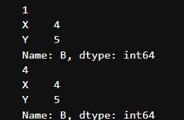
Here's a simplified and concise explanation of the output:

print(df.loc['X', 'A']):

• The output is 1, which is the value at row 'X' and column 'A

print(df.loc[['X', 'Y'], 'B']):

• It represents the values at rows 'X' and 'Y' for column 'B'.

print(df.iloc[0, 1]):

• The output is 4, which is the value at the first row(0th index) and second column(1st index i.e Column B).

print(df.iloc[[0, 1], 1]):

• It represents the values at the first two rows for the second column

Merging, joining, and concatenating :

1. Merging DataFrames:

   • Merging combines two or more DataFrames based on a common column (or columns) called a "key."

   • You can use the merge() function in pandas to perform merging.

Example of merging DataFrames:

# Create two sample DataFrames
df1 = pd.DataFrame({'key': ['A', 'B', 'C'], 'value1': [1, 2, 3]})
df2 = pd.DataFrame({'key': ['B', 'C', 'D'], 'value2': [4, 5, 6]})

# Merge the DataFrames based on the 'key' column
merged_df = pd.merge(df1, df2, on='key')

print(merged_df)

The output of merging example:

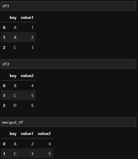
In the above example, we have two DataFrames (df1 and df2) with a common 'key' column. By merging them on the 'key' column, we create a new DataFrame (merged_df) that includes rows with matching keys from both DataFrames.

1. Joining DataFrames:

   • Joining DataFrames combines them based on their index values instead of a common column.

   • It is useful when you want to combine DataFrames based on their row index.

   • You can use the join() method in pandas to perform joining.

Example of joining DataFrames:

# Create two sample DataFrames
df1 = pd.DataFrame({'A': [1, 2, 3], 'B': [4, 5, 6]}, index=['X', 'Y', 'Z'])
df2 = pd.DataFrame({'C': [7, 8, 9], 'D': [10, 11, 12]}, index=['X', 'Y', 'Z'])

# Join the DataFrames based on their index
joined_df = df1.join(df2)

print(joined_df)

The output of joining example:

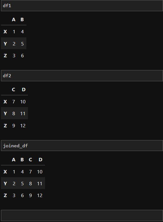
In the above example, we have two DataFrames (df1 and df2) with the same index. By joining them, we create a new DataFrame (joined_df) where the columns from both DataFrames are combined based on the shared index.

1. Concatenating DataFrames:

   • Concatenating DataFrames combines them along a particular axis (either rows or columns).

   • It is useful when you want to stack DataFrames vertically or horizontally.

   • You can use the concat() function in pandas to perform concatenation.

Example of concatenating DataFrames:

# Create two sample DataFrames
df1 = pd.DataFrame({'A': [1, 2, 3], 'B': [4, 5, 6]})
df2 = pd.DataFrame({'A': [7, 8, 9], 'B': [10, 11, 12]})

# Concatenate the DataFrames vertically (along rows)
concatenated_df = pd.concat([df1, df2])

print(concatenated_df)

The output of joining example:

In the above example, we have two DataFrames (df1 and df2) with the same column names. By concatenating them vertically, we stack the rows of df2 below df1 to create a new DataFrame (concatenated_df).

Statistical analysis

Various statistical operations that can be performed on a DataFrame in pandas:

1. mean():

   • The mean() function calculates the average value of each column in a DataFrame.

   • It computes the arithmetic mean by summing all values and dividing by the total number of values.

2. median():

   • The median() function calculates the middle value of each column in a DataFrame.

   • It finds the value that separates the higher half from the lower half of the data.

3. mode():

   • The mode() function identifies the most frequently occurring value(s) in each column of a DataFrame.

   • It returns a Series with the mode(s) for each column, as there can be multiple modes.

4. sum():

   • The sum() function adds up the values in each column of a DataFrame.

   • It returns the sum of all values, either for each column or for a specified axis.

5. max():

   • The max() function finds the maximum value in each column of a DataFrame.

   • It returns the highest value present.

6. min():

   • The min() function finds the minimum value in each column of a DataFrame.

These statistical operations can be applied to the DataFrame as a whole or to specific columns. Here's an example to demonstrate the usage of these functions:

df = pd.DataFrame({'A': [1, 2, 3, 4, 5],
                   'B': [2, 4, 6, 8, 10],
                   'C': [1, 3, 5, 7, 9]})

# Calculate mean
print(df.mean())

# Calculate median
print(df.median())

# Calculate mode
print(df.mode())

# Calculate sum
print(df.sum())

# Find maximum value
print(df.max())

# Find minimum value
print(df.min())

Window Functions:

Window functions in pandas operate on a specified window, Think of a window as a subset of rows that moves along as calculations are performed. This sliding window concept allows us to analyze data in a dynamic and flexible manner.

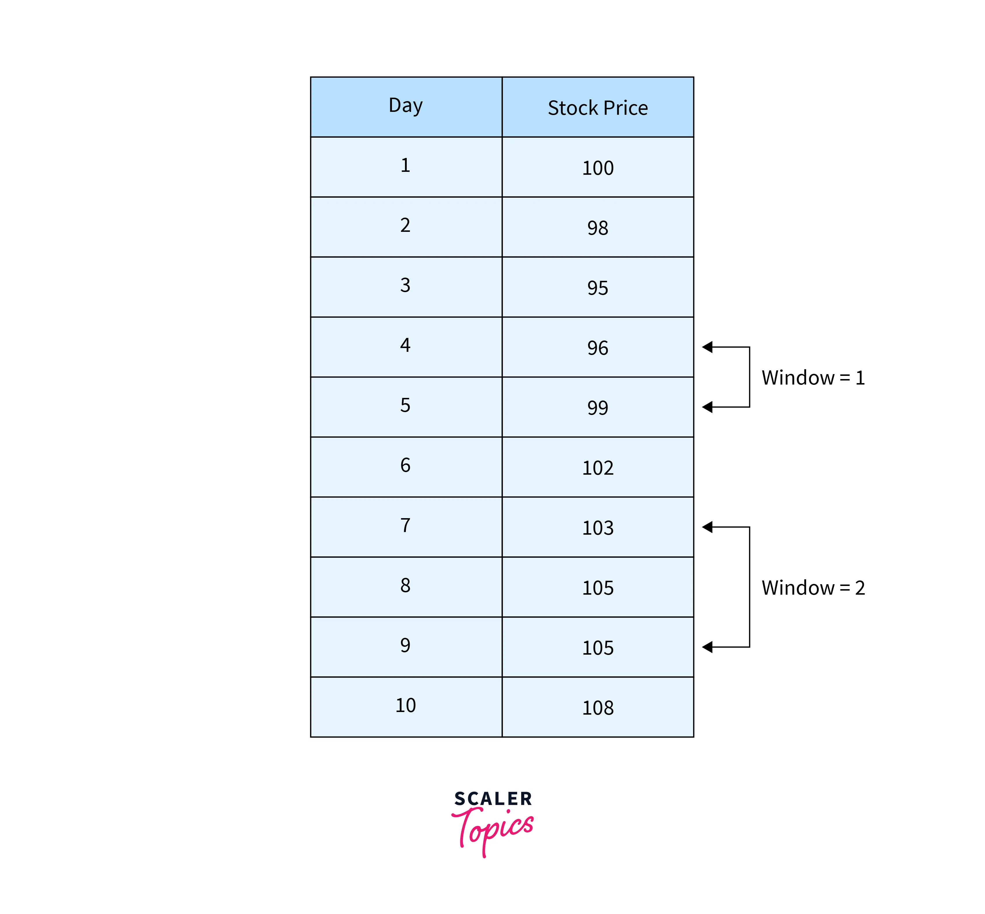
To access the window functions in pandas, we utilize the rolling() method, which creates a rolling window object. This object provides the foundation for applying different operations or calculations to the data within the window. Let's delve into some commonly used window functions :

1. Rolling Mean:

   The rolling().mean() function calculates the centered rolling mean within the window. This function is handy for smoothing out variations and identifying trends in time series data.

2. Rolling Sum:

   The rolling().sum() function computes the centered rolling sum, which provides insights into cumulative trends or accumulations within the data.

3. Rolling Maximum and Minimum:

   The rolling().max() and rolling().min() functions determine the centered rolling maximum and minimum values within the window, respectively.

4. Rolling Standard Deviation:

   The rolling().std() function calculates the centered rolling standard deviation, providing a measure of dispersion or volatility within the data.

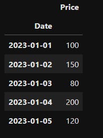
Let's illustrate the application of these window functions with a simple example. Suppose we have a DataFrame representing daily stock prices:

data = {'Date': ['2023-01-01', '2023-01-02', '2023-01-03', '2023-01-04', '2023-01-05'],
        'Price': [100, 150, 80, 200, 120]}
df = pd.DataFrame(data)
df['Date'] = pd.to_datetime(df['Date'])
df.set_index('Date')

Output dataframe:

To calculate the centered rolling mean, centered rolling sum, and centered rolling standard deviation over a window of 3 days, we can use the following code:

rolling_mean = df['Price'].rolling(window=3).mean()
rolling_sum = df['Price'].rolling(window=3).sum()
rolling_std = df['Price'].rolling(window=3).std()

Let's break down the code step by step:

1. rolling_mean = df['Price'].rolling(window=3).mean()

   • Here, we calculate the rolling mean of the 'Price' column in the DataFrame df.

   • rolling(window=3) specifies that the window size is 3, meaning we consider the current value and the two previous values.

2. rolling_sum = df['Price'].rolling(window=3).sum()

   • This line calculates the rolling sum of the 'Price' column in df.

   • Similar to before, rolling(window=3) defines a window size of 3.

3. rolling_std = df['Price'].rolling(window=3).std()

   • Here, we calculate the rolling standard deviation of the 'Price' column in df.

   • Once again, rolling(window=3) sets the window size to 3.

Data visualization in Pandas:

Pandas library offers a powerful built-in plotting functionality to effectively visualize data. By leveraging the .plot() method, you can create a variety of plots directly from pandas objects such as DataFrames and Series. This plotting functionality is seamlessly integrated with the Matplotlib library, providing customization options for your visualizations.

Suppose we have a DataFrame called sales_data that contains information about monthly sales figures for different products:

# Create a sample DataFrame
data = {'Month': ['Jan', 'Feb', 'Mar', 'Apr', 'May'],
        'ProductA': [1000, 1500, 1200, 1800, 1300],
        'ProductB': [800, 1200, 900, 1500, 1100]}
sales_data = pd.DataFrame(data)

The DataFrame sales_data looks like this:

Now, let's visualize this data using pandas' plotting capabilities:

1. Line Plot: We can create a line plot to visualize the monthly sales trends for both ProductA and ProductB:

sales_data.plot(x='Month', y=['ProductA', 'ProductB'], kind='line')

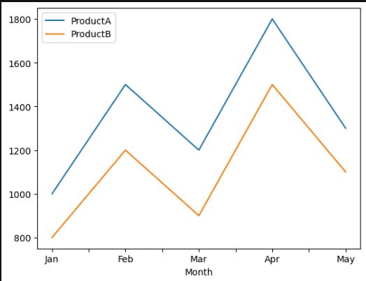
The line plot displays the sales figures over the months, with each product represented by a different line.

1. Bar Plot: To compare the total sales for each product across different months, we can use a bar plot:

sales_data.plot(x='Month', y=['ProductA', 'ProductB'], kind='bar')

The bar plot presents the total sales for ProductA and ProductB side by side, allowing for easy comparison.

1. Scatter Plot: Suppose we want to explore the relationship between ProductA and ProductB sales. We can create a scatter plot:

sales_data.plot(x='ProductA', y='ProductB', kind='scatter')

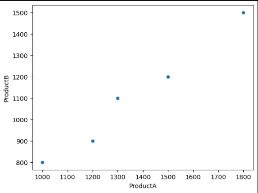
The scatter plot visualizes the correlation between the sales figures of ProductA and ProductB, with each data point representing a specific month.

These are just a few examples of the plotting capabilities provided by pandas. You can further customize the plots by adding titles, labels, legends, adjusting colors, and more. Additionally, pandas integrates with other libraries such as Matplotlib, allowing for even more advanced and specialized visualizations.

Summary

In short, the pandas library is a powerful tool for data manipulation, analysis, and visualization in Python. It offers intuitive data structures, efficient data operations, seamless integration with other libraries, and comprehensive data visualization capabilities. Pandas is an essential tool for data professionals, providing a seamless workflow for working with structured data and gaining valuable insights.